
Most experimental work in the life sciences already follows an iterative pattern. Whether the goal is making an assay more robust, finding a better therapeutic candidate, or improving a cell culture process, teams run rounds of experiments, look at the results, and decide what to try next. But the learning between rounds usually lives in notebooks, spreadsheets, and the scientists' heads. The rounds exist, but the feedback loop is still largely manual.
That becomes a real limitation when the relevant evidence does not arrive all at once. Some signals are available within hours. Others take days, weeks, or months. At any given point in a project, the next decision has to be made on incomplete information.
Closed-loop learning makes that feedback loop explicit. After and even during each round, the system updates its understanding of what looks promising, what remains uncertain, and which next experiments are most worth running. It does not require every candidate to be fully characterized before it can learn. It works with the evidence available now, refines its understanding as the missing pieces arrive later, and proposes the next batch of experiments and compiles them for the lab's automation hardware.
The core loop
At the simplest level, a closed loop does four things over and over:
- Run a batch of candidates.[1]
- Collect whatever evidence becomes available, from assay readouts to QC data, device logs, or characterization results.
- Update the model using both current observations and remaining uncertainty.
- Choose the next batch, while continuing to fold in slower signals as they arrive.
This is where it gets interesting. The system does not only ask where do I expect the best result? It also asks where am I still most uncertain? and where would another experiment be most informative? Balancing these questions is what makes the process adaptive rather than static. Early rounds are often broader, mapping the space and revealing where outcomes are sensitive to certain variables. Later rounds become more selective, focusing on the regions that matter most for the decision at hand. And crucially, the loop does not pause while waiting for slower data. It keeps moving with what it has and refines its understanding as delayed signals come in.
The number of experiments required depends on the biological system, measurement quality, and objective. Adaptive methods can help prioritize which candidates to evaluate. A design space with ten parameters at three levels each contains nearly 60,000 combinations, far too many to test exhaustively. Three families of methods address this:
- Design of Experiments (DoE) picks a structured subset of conditions up front, often a few hundred runs, giving controlled coverage and statistical rigor that unstructured manual exploration does not.
- Bayesian optimization can be seen as an iterative form of DoE: instead of fixing the full plan in advance, it updates a model after each round and proposes the next conditions, which makes it more sample-efficient on a single, well-defined objective.
- Active learning generalizes this further. It integrates a broader range of machine learning techniques, handles delayed and heterogeneous data types in the same project, and can learn from less explicit goal definitions, for example a target described in natural language or an example of a desired outcome rather than a hand-written scoring function.
ProviGen’s approach focuses on this last category: connecting active learning with experimental execution.
Assay optimization
An assay can be functional without being ready for routine use. Coefficient of variation (CV) is too high, edge effects appear unpredictably, or the protocol becomes fragile at scale. The usual fix is manual tweaking: adjust one variable, rerun, inspect, repeat.
In a closed-loop project, the team defines which parameters may vary and what “better” means: lower CV, higher Z′, stable signal separation, or lower reagent cost. That last one matters more than it may seem: a protocol that delivers reliable results at lower cost per plate can save significant budget when the assay runs at scale.
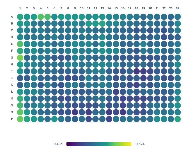
Each candidate is not a single well but a full assay condition with controls and replicates across a plate. A single well cannot tell you whether CV is acceptable, whether edge effects are under control, or whether the signal remains consistent across well positions. Those are plate-level properties, and they require plate-level evaluation.
Beyond the assay results, the system can incorporate execution context: dispense timing, shaker behavior, temperature drift, plate position effects, or environmental conditions. Over successive rounds, this reveals whether robustness problems are driven by the protocol itself or by specific execution patterns. The result is a clearer picture of why certain conditions fail and what operating ranges are safe to rely on.
Therapeutic design
In therapeutics design, the bottleneck is rarely lack of data. It is that the most meaningful data often arrives last. Binding, potency, and stability can be measured in vitro, while in vivo readouts may take weeks, months, or even years.
A closed-loop project starts with a broad first batch of candidates covering diverse regions of the design space. These are characterized through an initial panel of assays: binding, potency, stability. Even before any in vivo work has started, the model learns something useful. It may find that a region of the design space consistently lacks stability, or that certain candidates show a favorable potency-stability tradeoff.
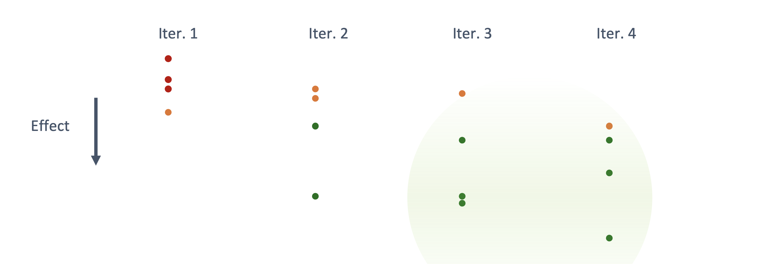
A subset of candidates then advances into more expensive downstream studies, including in vivo work. The loop does not pause. It keeps learning from the faster assay layers while delayed data is pending.
When in vivo results eventually arrive, they are linked back to the same candidates that already have characterization data. Now the model can do something much more valuable than marking winners and losers: it starts learning which early signals actually predict downstream performance and which ones were misleading. Future candidate selection shifts accordingly, guided less by proxy performance alone and more by the patterns that genuinely translate.
Media formulation
Media formulation is rarely about one magic ingredient. Performance typically emerges from interactions between basal media, supplements, growth factors, cytokines, and timing decisions. Even with just a handful of variables, the number of possible combinations is far too large to screen exhaustively, and formulations are often constrained (for example, the fractions of a blend must sum to one).
A closed-loop project starts broad: the first round covers a wide range of compositions, each run with replicates. As results come in, the system collects whatever evidence is available, from cell counts and viability to process traces and environmental conditions, and updates its model without waiting for every candidate to be fully characterized.
The next set of conditions balances candidates likely to improve the target outcome against ones that would resolve open questions about interactions. For example, whether two basal media compensate for each other when blended, or whether a cytokine only helps when paired with another.
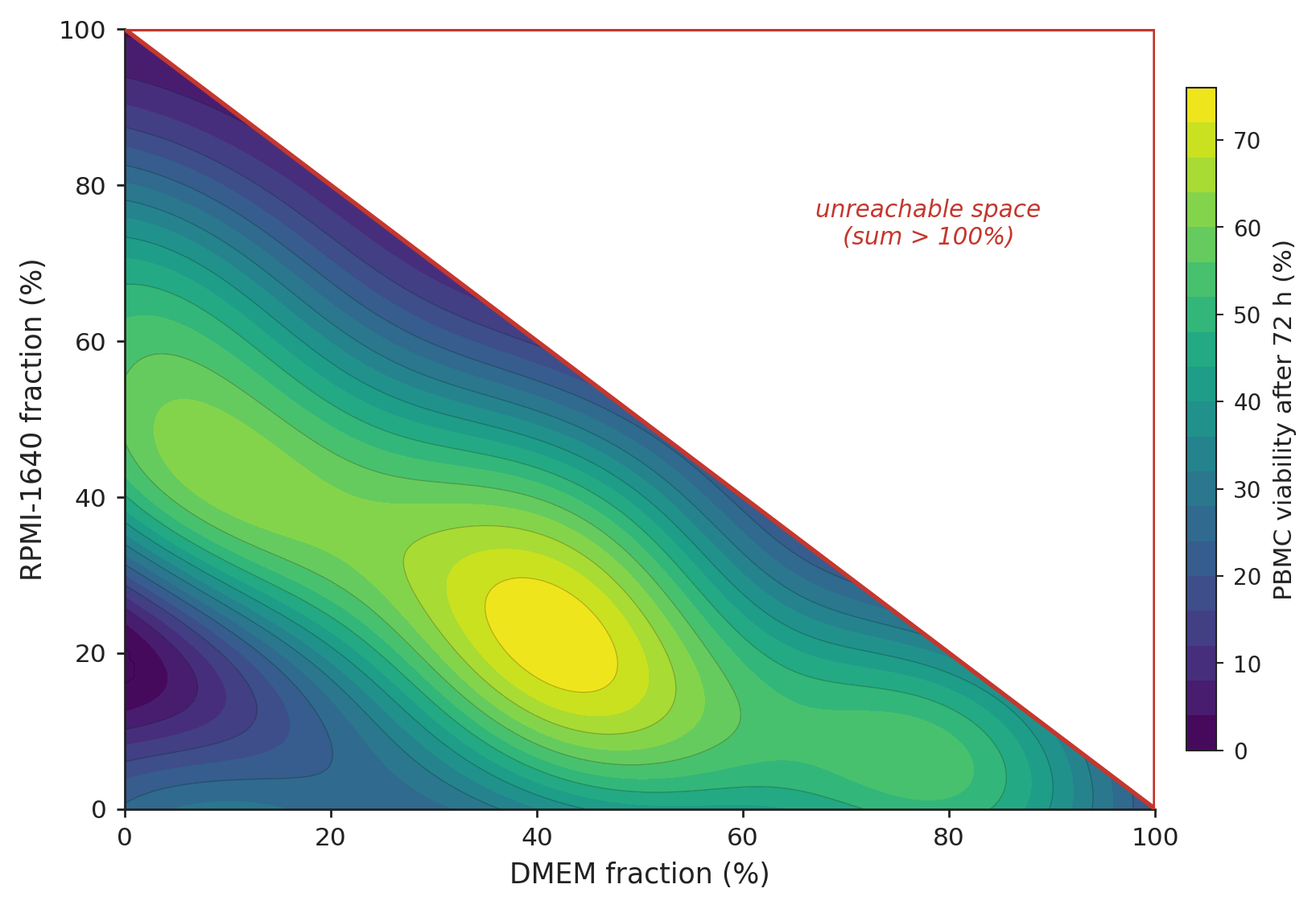
Over successive rounds, the loop builds up a picture of the formulation space. You learn that a specific blend of commercial media outperforms any single one, that a cytokine cocktail preserves the balance of cell subpopulations better than standard mixes, or that a growth factor can be halved without losing viability. That understanding is what makes a protocol transferable and reliable at scale.
What counts as a sample?
A “sample” in a closed-loop project is the decision unit being evaluated, not necessarily the smallest physical unit in the lab.
In assay optimization, that may be a full assay condition summarized across a plate layout. In therapeutic design, it is often a candidate variant or variant-condition pair. In media optimization, it is typically one media or process condition evaluated with replicates.
The important point is that the sample follows the decision boundary, not the instrument boundary. Replicates strengthen confidence in that evaluation, but they do not redefine what the candidate is.
| Application | What varies | One sample | Data sources |
|---|---|---|---|
| Assay optimization | Timing, concentrations, volumes, plate handling | Condition at plate level | Well readouts, replicates, device logs, environmental data |
| Therapeutic design | Sequence, structure, modifications | Candidate with multi-stage data | In vitro screens, stability, delayed in vivo data |
| Media formulation | Composition, supplements, feeding schedule | Condition with replicates | Replicate wells/flasks, time-course, metabolic readouts |
Status: experiment design, running. Our active learning system is built for cases where standard Bayesian optimization struggles: multiple objectives, heterogeneous data sources (assay readouts, QC, analytics, in vivo), and signals that arrive on very different timescales. It learns how those sources relate to each other and to the outcomes that matter, which is what allows it to make useful decisions even when some signals are missing, delayed by months, or structurally different from each other.
From the user's perspective: you define what you want to achieve; the system proposes the next round and compiles it into an instrument program (running for supported workflows); scheduling and execution are in development; a scientist approves every batch. The complexity lives underneath. It surfaces as decisions a scientist can trace back to the evidence behind them.
If you are interested in exploring what a closed-loop project could look like for your workflow, start a research conversation.
[1] In a fully closed-loop setup, running a batch means generating the protocols, scheduling the instruments, and capturing the resulting data automatically. It is designed for instrumentation that supports programmatic control, including liquid handlers, plate readers, and incubators, whether driven through vendor APIs, a scheduling layer, or open-source frameworks like PyLabRobot; each instrument is integrated individually. At ProviGen, protocol compilation runs for supported workflows; scheduling and execution are in development.
[2] A simulation, computed in your browser as you read. The landscape is the Branin function, a standard benchmark for optimization methods with three equally good minima. Left, a Latin hypercube: a space-filling design fixed before the first experiment. Right, after three spread-out starts, a Gaussian-process model is refitted to every measurement and places the next experiment where its expected improvement is highest (Jones, Schonlau & Welch 1998), in the form for noisy measurements (Huang et al. 2006). Every measurement carries random noise of 2% of the function's range; the strip tracks the true value of the best experiment so far, on a log scale. Each run draws a new design and new noise, and the outcome varies: over many runs the experiments chosen one at a time usually, but not always, end closer to the optimum, and the first run shown is a typical one. The figure shows the principle on a smooth function of two inputs. It is not lab data, and it says nothing about how any method performs on a real assay.
[3] Response surface fit via Gaussian process regression to 24 experimental points from the PBMC media-blending study in Narayanan et al., “Accelerating cell culture media development using Bayesian optimization-based iterative experimental design,” Nat. Commun. 2025, which reports higher sample efficiency than classical Design of Experiments across both the PBMC and recombinant-protein studies. Source data: figshare 27715134.
References and credits
- 01Narayanan et al. · Accelerating cell culture media development using Bayesian optimization-based iterative experimental design · Nature Communications · 2025External. The media example reconstructs this published study; attributed literature evidence, not a ProviGen result. Source data: figshare 27715134.
- 02Surjanovic & Bingham · Branin function · Virtual Library of Simulation Experiments: Test Functions and Datasets · Simon Fraser UniversityExternal. Definition, domain and minima of the test function the simulation runs on.
- 03PyLabRobot · open-source laboratory automation frameworkExternal. One of the open frameworks through which instruments can be driven programmatically.
- 04Original publication · ProviGen field noteFirst published April 2026.